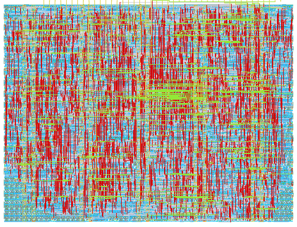
130 PQN Model with Verilog
130 : PQN Model with Verilog

- Author: kinako71-2
- Description: ASIC implementation of a PQN model with two variations that can generate class 1 and class 2 firing patterns.
- GitHub repository
- Open in 3D viewer
- Clock: 5000000 Hz
How it Works
This project is based on the PQN model[^1], which is designed for the digital implementation of neuron circuits.
In particular, this work adopts a two-variation PQN model.
The parameters are configured to reproduce Class 1 and Class 2 neurons according to Hodgkin’s classification[^2].
Governing Equations
Following footnote 1, The neuron dynamics are defined as:
\frac{dv}{dt} = \frac{\phi}{\tau} \left( f(v) - n + I_0 + k I_{\text{stim}} \right)
\frac{dn}{dt} = \frac{1}{\tau} \left( g(v) - n \right)
f(v) =
\begin{cases}
a_{fn}(v - b_{fn})^2 + c_{fn} & (v < 0) \\
a_{fp}(v - b_{fp})^2 + c_{fp} & (v \ge 0)
\end{cases}
g(v) =
\begin{cases}
a_{gn}(v - b_{gn})^2 + c_{gn} & (v < r_g) \\
a_{gp}(v - b_{gp})^2 + c_{gp} & (v \ge r_g)
\end{cases}
b_{fp} = \frac{a_{fn} b_{fn}}{a_{fp}}
c_{fp} = a_{fn} b_{fn}^2 + c_{fn} - a_{fp} b_{fp}^2
b_{gp} = r_g - \frac{a_{gn} (r_g - b_{gn})}{a_{gp}}
c_{gp} = a_{gn}(r_g - b_{gn})^2 + c_{gn} - a_{gp}(r_g - b_{gp})^2
To reduce the computational cost, each coefficient is expanded in the implementation. Here equations are expressed as follows:
\frac{dv}{dt} =
\begin{cases}
f_{vv_n} v^2 + f_{vv_n} v + f_{\text{const}_n} - f_{\text{coef}} n + I_{\text{coef}} I_{\text{stim}} & (v < 0 ) \\
f_{vv_p} v^2 + f_{vv_p} p + f_{\text{const}_p} - f_{\text{coef}} n + I_{\text{coef}} I_{\text{stim}} & (v \ge 0)
\end{cases}
\frac{dn}{dt} =
\begin{cases}
g_{vv_n} v^2 + g_{vv_n} v + g_{\text{const}_n} - g_{\text{coef}} n & (v < r_g) \\
g_{vv_p} v^2 + g_{vv_p} p + g_{\text{const}_p} - g_{\text{coef}} n & (v \ge r_g)
\end{cases}
Parameter Configuration
Below are the detailed values of the parameters.
For the expanded coefficients used in implementation, please refer to the module script for detailed values.
| Parameter | class1 | class2 |
|---|---|---|
| $dt$ | 0.0001 | 0.0001 |
| $a_{fp}$ | -3.5 | -4 |
| $a_{fn}$ | 3.5 | 4 |
| $b_{fn}$ | -2 | -2 |
| $c_{fn}$ | 0.5 | 5.25 |
| $a_{gn}$ | -0.5 | -3 |
| $a_{gp}$ | 2.5 | 3 |
| $b_{gn}$ | -3 | -2 |
| $c_{gn}$ | -16 | -16 |
| $\tau$ | 0.0064 | 0.0064 |
| $I_0$ | -16 | -16 |
| $k$ | 8 | 8 |
| $\phi$ | 0.125 | 0.125 |
| $r_g$ | -2.5 | -2.5 |
Module Interface
The ports usage of the top module is as follows:
| Pins | Bits | Direction | Description |
|---|---|---|---|
clk |
1 | Input | Clock signal |
rst_n |
1 | Input | Active-low reset signal |
uio_oe[7:0] |
8 | Input | Set to 1 to enable outputs at all times |
ui_in[7:1] |
7 | Input | Input current, converted to 16 bits |
ui_in[0] |
1 | Input | Mode select input |
uo_out[7:0], uio_out[7:0] |
16 | Output | Signed 16-bit membrane voltage |
[^1]: Nanami, T., & Kohno, T. (2023). Piecewise quadratic neuron model: A tool for close-to-biology spiking neuronal network simulation on dedicated hardware. Frontiers in Neuroscience, 16, 1069133.c
[^2]: Hodgkin, A. L. (1948). The local electric changes associated with repetitive action in a non-medullated axon. The Journal of physiology, 107(2), 165.
How to Test
Simulation was originally conducted using Julia.
The given inputs and the corresponding ideal outputs are provided as text files (ans_* and input_*, where * = class1 or class2).
The test bench checks whether the circuit reproduces these results.
Please note that each output point is generated every 18 × 10 clock cycles.
External Hardware
A PCB board is sufficient.
IO
| # | Input | Output | Bidirectional |
|---|---|---|---|
| 0 | Mode Select (0: Class 1, 1: Class 2) | Membrane Potential [0] | Membrane Potential [8] |
| 1 | Input Current [5] | Membrane Potential [1] | Membrane Potential [9] |
| 2 | Input Current [6] | Membrane Potential [2] | Membrane Potential [10] |
| 3 | Input Current [7] | Membrane Potential [3] | Membrane Potential [11] |
| 4 | Input Current [8] | Membrane Potential [4] | Membrane Potential [12] |
| 5 | Input Current [9] | Membrane Potential [5] | Membrane Potential [13] |
| 6 | Input Current [10] | Membrane Potential [6] | Membrane Potential [14] |
| 7 | Input Current [11] | Membrane Potential [7] | Membrane Potential [15] |